CS 6601: Artificial Intelligence
CS 6601 Artificial Intelligence
Preamble
Hey! This is my first course of the Georgia Tech’s OMSCS program. This document is an attempt to sythetize the course material for future reference, as well as to keep a trace of my learning for future reflections.
Why CS 6601 AI? With my BMath being in Stats, I saw a lot of theory and classical ML techniques. I am hoping to gain a better understanding of the field of AI as a whole through this course, as well as improve my ability to implement algorithms from texts. From the reviews I found on Reddit, OMSHub and OMSCentral, this course looks like the perfect place to gain a deeper understanding of AI techniques.
My perceived strengths before starting:
- My mathematical background. I believe it will help me grasp quicker the theoretical aspects of the techniques.
- My interest: I really enjoy learning and applying algorithms, so I believe the extra motivation will be a great plus.
- Work experience: I use Python every day at work and have implemented non-AI algorithms from scratch in my professional experience.
My perceived weaknesses before starting:
- Coding speed: While I code every day at work, I am impressed by the amount of content that it looks like we will be covering during the course. My coding will be challenged for sure.
- Lack of a network: As this is my first class, I do not know anyone in class or currently in the program to share my struggles with. My goal is to be active on the course forums to maybe build such connections, or at least enjoy some participation.
- Readings: There seems to be a lot of assigned readings. As I stare at screens so much already, my fear is that I get exhausted from them - but I ordered a physical copy of the book which will hopefully help.
Course Reviews Metrics
- OMSHub:
- Rating: 4.1/5
- Difficulty: 4.0/5
- Workload: 22.6 hrs/week
- Number of reviews: 241
- OMSCentral:
- Rating: 4.08/5
- Difficulty: 4.08/5
- Workload: 23.01 hrs/week
- Number of reviews: 264
The syllabus is publicly available: Link Textbook: Artificial Intelligence: A Modern Approach (4th Edition)
My Review
TBD at the end of the course…
What went well:
- The Discord Channel was a lifesaver. The lack of a network ended up being moot. With over 600 students in the class, there’s a lot of opportunities to support others and get support.
- Math background definitely helped. No proofs, but there was a lot of readings, equations to translate/understand, etc.
- Each week I checked how many pages we had to read, and the length of the lecture videos, and I managed to stay on schedule by splitting them by the number of days in the week.
- I tackled a lot of the assignments before the 2nd weekend, by front loading my efforts. This allowed me to get some less hectic weeks every 2-3 weeks, focused on readings and lectures.
What went wrong:
- I spent over 50 hours on the first assignment, and as result I got a little burnt out by the time the 3rd assignment rolled around, because this course doesn’t give a lot of time to breath, until later on.
- Speaking of, there were a few weeks with a LOT of readings assigned, where I would have been better served to mix it with doing quiz questions.The quizzes were extremely helpful.
- With scoring successes on the first 5 assignments, I decided to skip assignment 6 for my mental health. TBD if this was a mistake for the final. My rating: 5/5 My difficulty: 3.5/5 My workload: 15 hrs/week Next Steps: TBD
Overall, I’m very happy to have taken this course as my first one in the program. The excitment from starting a new journey paired well with the front-load of the course, and my undergrad in Stats paired really well with the more difficult material. I found the first assignment extremely challenging, but then something clicked. The book and supplemental material were very useful, as well as the community of students and instructors on Ed ad Discord. It really reinforced into me that I am much better at learning while doing, and that is what I will be prioritizing in future courses.
On workload: Until week 5, I was averaging 19 hours per week on the course, but this number is skewed higher by working 30 hours on the 2nd week of A1. After that, I didn’t keep track, but I would be surprised if I worked more than 15 hours on any given week outside the midterm week - probably thanks to having a background in Stats too.
- Search
1. Search
(Chapter 3 in textbook)
Agents used to solve search problems are called Problem Solving agents, and they act in simple environments: episodic, single agent, fully observable, deterministic, static, discrete and known.
An agent follows 4 phases of problem solving:
- Goal Formulation: Sets a clear objective
- Problem Formulation: Which actions can be taken to solve the problem? How will they affect the state of the world?
- Search: Simulate actions to find a solution ( a sequence of actions that reaches the goal)
- Execution: Perform the actions one after the other
Our problem-solving agent operates in an open-loop system.
What is the problem we are trying to solve? We are trying to find shortest paths, without knowing every possible route.
Example of a problem Finding the shortest path from Toronto to Montreal.
Definition of a problem
-
State Space: A set of states (s) that the environment can be in (eg. we can be in a city in Ontario).
-
Initial State (eg. starting in Toronto)
-
Goal States: The goal(s). It can be only one, but it can also be a set of goals. It can also be defined by a property that applies to many states (ie. all plates are empty of food)
-
Action(s): Takes inputs and return a set of possible actions $${a_1, a_2, a_3, … ,a_n}$$
-
A transition model, or Result function: $$ Result(s,a) -> s’$$ where s: state, a: action and output is new state.
-
Goaltest function: To test if we reached our goal $$ GoalTest(s) -> T | F$$
-
PathCost function: Takes a sequence of states/actions and returns the cost of the path n. $$PathCost(s->^a s->^a s->^a… ->^a s) -> n $$ $$StepCost(s,a,s’) -> n_a$$
Path: Sequence of ActionsSolution: A path from the initial state to a goal stateOptimal solution: The path with the lowest cost amonst all solutions.At this point, assumption is that all costs are positive.
A graph to represent the state pace can be thought of by using vertices to represent the states, and directed edges between being the actions.
(We say it’s a graph search when looking for redundant paths, and a tree search if no)
We represent the problem through abstraction, which aims to reduce the amount of details to the minimum necessary to act on the problem easily.
The state space describes all the possible states of the world. While the search tree describest the paths between the states, to the goal.
One state might appear in multiple branches of the tree, as the state can be reached through multiple paths. However, each (path) has a unique path to its root.
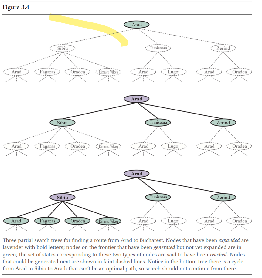
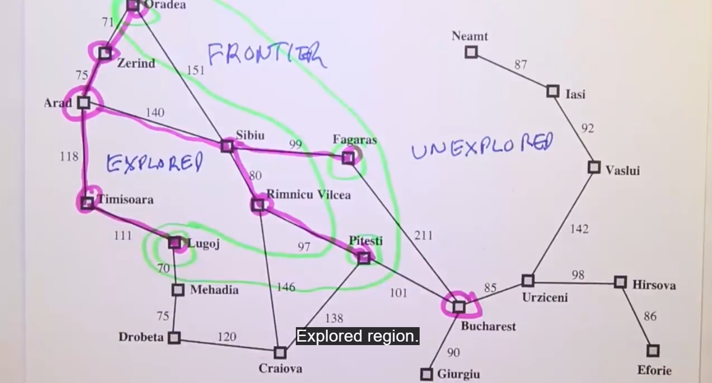
Every node in the frontier or in the explored region is considered reached.
A node is considered expanded if it has been reached and we used the result function to see where the actions lead and we generate a new node to represnet each resulting state.
Search Data Structures (Implementation)
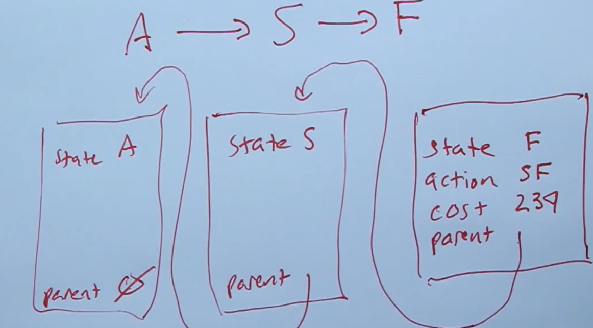
Node is a data structure with 4 components:
- node.State: The state related to the node
- node.Parent
- node.Action: The action from the parent state to this node.
- node.path-cost: The cumulative sum of the path from the root node to this node.
 Frontier with operations:
 - is-empty: to check whether the frontier is empty or not?
- pop: Removes the top node from the frontier and returns it.
- top: Only returns the top node of the frontier
- add: Insert the node
- Usually a Priority Queue (PQ) and/or set (or hash table)
Explored List
- Set (hash table)
Usually frontier is implemented by using a queue (priority queue, FIFO, LIFO).
The reached state is usually stored using a key-value (state-node) lookup table - like a hash table.
How to avoid cycles?
- Keep a history of previously reached states.
- Good for: Many redundant paths
- Pros: Never reach a redundant path
- Cons: Takes a lot of memory
- Not worry about the past
- Good for: When redudant paths are not a worry, or a very rare worry.
- Pros: No additional memory cost.
- Cons: Could stumble upon a redundant path if not careful.
- Check for cycles, not redundant paths by using the parent pointers to check if the node appeared previously.
- Good for:
- Pros: Eliminates all cycles of lengt l
- Cons: Computing time
Algorithms
Evaluation Evaluate search algorithms using four criteria:
The depth is the number of actions in an optimal solution, and a m is the max number of actions in paths. b is the branching factor (# of successors of a node that need to be considered).
1.0 Best-first Search
For n being a node on the frontier, and f(n) being a an evaluation function that calculates the cost of going to node n.
We want to expand to the node on the frontier with the minimum value of the evaluation function f(n).
Then add each child node generated by the expansion to the frontier. But only add those that haven’t been reached before, and re-add those that have been reached before, but now have a smaller cost (value of f(n)).
Uninformed Search strategies
The following search algorithms are “uninformed”. They have no clue how far the goal(s) is from the state.
1.1 Breadth First Search
(shortest-first search)
- Good when all actions have equal cost.
- Complete (even on infinite state space).
- Searches depth by depth
- f(n) is the depth of the node -> always pick the path with shortest depth.
- FIFO queue
- reached set can be states directly
- Early goal test (check whether node is a solution as soon as it’s generated)
- Complexity (tim and space): $$ O(b^d) $$ Where b are successors, and d is depth
1.2 Uniform Cost Search
(Dijkstra’s algorithm) (cheapest-first search)
- Good when all actions have different costs
- Searches by minimizing the path cost at each step.
- Worst-case time Complexity: C* is cost of the optimal solution, epsilon (e) is lower bound on the cost of each action, e > 0
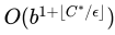
- If all costs are equal, the second term becomes depth
- Complete and cost-optimal
Head up: A star * means optimal.
1.3 Depth First Search
- f(n) is the negative of the depth.
- Does not keep a table of reached states (usually).
- Expands deepest nodes first.
- Not cost optimal, first solution found is returned.
- Incomplete: It might never terminate in an infinite state space.
- If cyclic state space, check for cycle before new node.
- Smaller memory need (other algorithms are very expensive). Small frontier and don’t keep track of reached states.
- Time complexity proportional to number of states.
- Memory complexity: b is branching factor, m is the max depth of tree $$ O(bm) $$
Depth-limited search is depth-first search where a limit exist to how deep we explore.
Cycles are handled by looking back up the chain a set amount of time, or by the depth limit.
Iterative Deepening combines depth-first and depth-limited searches. It starts with depth limit l = 0 to 1 to 2 … until it finds a solution or returns failure value.
Usually preferred when the search state space cannot fit in memory and we don’t know the depth of the solution.
1.4 Bi-Directional Search
- Simultaneously searches from the start to goal and from goal to start
- Keep track of two frontiers, two explored sets
- Solution exists when two frontiers collide
- Complete in finite state space and both directions a breadth-first or UCS
- Optimal under certain conditions (one possible being all the path costs being weighted the same)
Bi-Directional UCS
- Uses path cost as evaluation function
- Stop condition when the sum of both frontier’s priority is over the cost of the best path found
Bi-Directional A*
- Uses f(n) = g(n) + h(n) as evaluation function (look 1.5 A* Search below)
- Stop condition more complex: But can use the same as Bi-UCS
Informed (With Heuristics) Search Strategies
1.5 A* Search
- Cost optimal if admissible
- Complete
The A* search is similar to UCS, with the evaluation function: f(n) = g(n) + h(n), where g(n) is the cost of the path until node “n”, and h(n) is a heuristic function that estimates the cost from h(n) to the goal.
This helps the search to advance faster, while still being complete and optimal under the condition of admissibility, and stronger, the condition of consistency
Admissibility ensures optimality: Assume we find a path using the algorithm with admissible heuristic, but we missed a path of optimal cost. Since the heuristic is lower than the true cost of reaching the goal, this means that the algorithm didn’t expand this potential path, which would have been lower than the one we found.
That is, the algorithm is consistent if the heuristic cost from n to goal is smaller than the real cost from n to successor n’ + the heuristic cost from n’ to goal.
Every consistent heuristic is also admissible (but the reverse is not true).
Weighted A* Search
The heuristic becomes f(n) = g(n) + Wh(n) for W > 1. For optimal cost C, the solution found will be between C* and C* * W. A* has W=1, UCS has W=0 and Greedy has W = infinity
Beam Search:
Aims to save memory space by limiting the size of the frontier.
Iterative-Deepening A* Search (IDA*)
Brings together ideas from Iterative-Deepening and A* search, where the cutoff is the f-cost is the smallest f-cost of any node that exceeded the cutoff on the previous iteration.
IDA* works well when multiple path costs are the same, otherwise it could only increase the cutoff by 1 node each iteration and take a long time.
Finding Optimal Solutions to Rubik’s Cube Using Pattern Databases, Korf: Uses IDA* to solves Rubik’s cube.
Uses too little memory.
Recursive Best-First Search (RBFS)
(to review) Keeps track of alternative paths better than the current one, and recursively iterate until a certain f-value is exceeded. It is optimal if the heuristic used is admissible.
Uses too little memory. As in IDA*, could end up exploring the same node multiple times over.
Memory-Bounded A* (MA*)
Limits the memory usage of A* without compromising optimality as much as IDA* and RBFS.
Simplified Memory-Bounded A* (SMA*)
Similar to RBFS, except it makes use of more memory: It stops when the max memory is achieved, then uses all the information to delete the leaf node that is the worst (with highest f-value).
- Complete if the goal can be reached within memory limitations.
1.6 Greedy Best-First Search
Best first search with evaluation function f(n) = h(n) the heuristic function.
- Complete in finite state spaces
- Incomplete in infinite state spaces
- Worst time and space complexity O(|V|) - can be reduced to O(bm) with good h(n)
- Not guarantee of optimality
1.7 Bi-Directional A* Search
2 A* searches simultaneously: from front and from back. Manages two different frontiers and two different explored sets.
Consider other paths until the stopping condition is satisfied.
There are different possible stopping conditions. One of them is if the cost of the current path is smaller than all of (frontier_best_path_cost_forward + frontier_best_path_cost_reverse), priority_forward and priority_reverse.
Here are great resources for Bi-Directional algorithms:
- Bi-Directional Search, Ira Pohl: Explains and explores bi-directional algorithms, stopping conditions and their advantages/disadvantages.
- Efficient Point-to-Point Shortest Path Algorithms, Goldberg, Harrelson, Kaplan and Werneck: Slides that demonstrate pseudocode and stopping criterion for uni-directional UCS, A*, as well as their Bi-Directional versions.
1.8 A* with Landmarks (ALT Algorithm)
Computing the Shortest Path: A* Meets Graph Theory, Goldberg and Harrelson: Using pre-computed landmarks to help the A* algorithm be more efficient for real map applications.
The idea is to precompute paths from every node to a small subset of landmarks to obtain a better heuristic. Here are two different heuristics possible with this idea:
$$ 1. h_L(n) = min_{L \epsilon Landmarks} C^(n,L) + C^(L, goal) $$ $$ 1. h_{DH}(n) = max_{L \epsilon Landmarks} |C^(n,L) - C^(goal, L)| $$
The first one might be inadmissible if the optimal path doesn’t go through a landmark. The second one is admissible when the landmark is beyond the goal.
Selecting Landmarks can be done multiple ways: at random, or trying to sparead them apart as much as possible, etc.
1.9 Heuristic Functions and their Evaluations
Where
- N is the number of nodes generated by an algorithm (eg. A*)
- d is the depth of the solution
And b* is the branching factor required to obtain N+1 nodes. Closer to 1 is good.
Is h1(n) > h2(n) and both are admissible heuristics, we say that h1(n) is dominant over h2(n) -> it will always find the solution faster (or in the same amount of of nodes explored) when compared to using h2(n).
We can also generate heuristics programatically by removing conditions, which is called “relaxing” a problem.
Using a composite heuristic h(n) = max{h1(n), h2(n), … , hk(n)} results in a better heuristic than any of the heuristics individually, assuming they are all admissible.
2. Intelligent Agents
(chapter 2 in textbook)
Agent
They use atomic representations. That is,
Environment
3. Search in Complex Environments (incl. Simulated Annealing)
(Chapter 4 in texbook)
3.1 Local Search and Optimization Problems
Advantages:
- Low Memory requirements
- Find good solutions in big search state spaces
Hill Climbing Simple algorithm that will pick the direction of steepest ascent/descent to move to. It will stop when no neighboring state is higher/lower. It will also stop on a plateau (a flat space where the objective is not improved or diminished).
It can get stuck due to local maxima, ridges (a sequence of lcoal maxima) or plateaus.
Variants exist to find solutions to these issues:
- Allow sideways move on plateaus until a limit of n moves is crossed.
- Stochastic Hill Climbing is a probabilistic hill climbing method that will assign higher weights to steepest ascents, but leaves a chance to choose a less steep hill.
- First-choice Hill climbing: If too many neighbors are present and slowing down computation, check neighbors one by one at random. The first one to be better than current state is chosen.
- Random-Restart Hill Climbing: Restart hill climbing from a random starting point a bunch of times in the hope that you find the goal eventually. E(#Restart) = 1/p, where p is the probability that hill climbing will find a solution.
Simulated Annealing
Simulated annealing is designed so it is possible to go downhill, even when the goal is a maximization one. The reasoning behind it is avoid getting stuck in local maxima by allowing our agent to explore a different area in the state space that would otherwise not be possible under hill climbing.
It is similar to hill climbing, except that it chooses the next neighbor at random - and accepts it if it is going in a positive direction. If the neighbor is going in a negative direction, is is accepted with probability $$e^{(\Delta E/T)}$$ where delta E is the difference between our state and the neighbor (steepness of the “descent”). This will be negative since we are only looking at this probability if the neighbor is worst.
T is the “temperature” parameter, it is set by us to decrease over time. What it does is help dictate how likely it is to accept a bad move: Early on, the temperature is high (high entropy), we accept more bad moves. As time passes we assume that we are getting closer to a true maxima and thus reduce the chance of choosing a bad move.
Local Beam Search Keeps track of k states instead of one.
- Randomly generates k states
- Generate all successors of all k states
- Halts when find a goal
- If no goal found, select the k best successors from the complete list and repeat
Stochastic Beam Search helps making the successors not all clumped together by allowing some less good successor be chosen with a certain probability value (usually based on the value of the successor).
Evolutionary Algorithms These algorithms try to emulate the process of evolution in nature.
A starting population is generated (at random?), and the algorithm depends on multiple things:
- Mix according to a mixing number rho - how many parents to create an offspring (usually 2).
- Selection process to decide which are fit to become parents (can select via probability based on potential parent’s scores, or just pick the best n parents).
- Recombination procedure: for example, picking the first half of a path from one parent, then second half from the other.
- Mutation rate introduce some variability in the offsprings by introducing random changes in the parent’s “genes”
- The makeup of the next population: Decides which parents/children continue on.
3.2 Local Search in Continuous Spaces
Problems with continuous action spaces contain infinite branching, so we cannot handle them the same as discrete state spaces.
There are a few solutions to continuous state spaces. One of them is discretizing the space. That is, limiting the space to only a limited amount (size delta) of states.
We can also use random sampling to move avoid exploring each actions, but randomly explore states that improve our solution. These types of algorithms are called empirical gradient.
We can use calculus and derivatives to find the direction of steepest ascent/descent when we define our problem with a mathematical function.
Constrain Optimization problems are those where solutions must satisfy some constraints.
3.3 Search With Non-Deterministic Actions
This part deals with nondeterministic environments (the agent doesn’t know with certainty what the action it took will lead to).
AND-OR Search Trees In a deterministic environment, our agent knows that in a state, it can do one action OR another action. “OR NODES”.
In a non-deterministic environment, the result of these “OR NODES” can be different states, such that the agent will need to plan for state A AND state B “AND NODES”.
A solution to the AND-OR search tree is one that
- has a solution at each leaf node,
- Includes one action at each OR node and
- includes every outcome branch at each of its AND nodes
Cyclic solutions can exist when we need to repeat some action to achieve the goal with certainty. It is possible that the reason why we need to repeat is such that repeating the action will never gets us to the goal, but if there is a possibility of working, then at some point it will reach the goal.
3.4 Search in Partially Observable Environments
This section introduces Partially observable environments (the agent doesn’t know with certainty which state it is in).
Sensorless/Not Observable Environments
A Sensorless problem arises when the agent detects no information about the environment at all. Possible to solve under te right conditions.
One way to solve them is by coercing the agent in a (goal) state with certainty, by following a pattern of actions that will definitely find a solution.
We can use algorithms from Chapter 3 (Search) to solve sensorless problems, by using a belief-state model instead of a physical-state mdoel:
- States Contains every possible subset of the physical states. In a problem P with N states, the belief-state has 2^N belief states.
- Initial State: The belief state consisting of all states in P. But usually there are limited starting points that we know of
- Actions Either the union of all actions (if we can try illegal actions), or the intersection of actions that are legal in every state (if illegal actions are strictly forbidden)
- Transition Model: One result state per current possible state (deterministic actions), or the union of all possible results from actions on each current possible state (nondeterministic actions)
- Goal Test: We can possibly achieve the goal if any state s in the belief state is a goal state. And we necessarily achieve the goal state when every state satistifies the goal.
- Action Cost: Assume it can be transferred from the physical problem, but could get complicated if the cost depends on the state.
A different approach is to perform incremental belief-state search algorithms, in which we find a solution incrementally.
Partially Observable Environments
Adds a PERCEPT(s) function that returns what can the agent perceive in a certain state s. In a fully observable environemnt, Percept(s) = s everywhere. In a sensorless problem, Percept(s) = null everywhere. In a non-deterministic environment, Percept(s) = {s1, s2, …, sn} a list of all possible states.
A transition model between states in a partially observable environment has 3 stages:
- Prediction outputs the belief state resulting from taking an action. PREDICT(b,a) is a synonym to RESULT(b,a)
- Possible Percepts returns all the percepts that can be observed in the predicted belief state
- Update is computed for each possible percept. Outputs the belief state that would result from the percept.
Solving The transition model gives us a method to compute results. We can then use the AND-OR search algorithm to solve the problem.
Differences with an agent for fully deterministic and observable environments
- Solution will be a conditional plan, not a sequence
- Maintains a belief state as it navigates the solution
3.5 Online Search Agents and Unknown Environments
Good for when there is a penalty for sitting around too long. Or for nondeterministic domains, so that we can focus on what happens rather than things that might happen and waste a lot of computation.
The agent knows the following:
-
Actions(s): The legal actions in state s
-
c(s, a ,s’) the cost of action a from s to s’ -> only once agent knows that s’ is an outcome
-
Is-Goal(s): Testing for the goal
Competitive Ratio: The ratio between the cost of the optimal path and the cost that the agent incurred via travelling the online problem.Safely Explorable: A goal state is reachable from every reachable state.
To discover children/neighbors/successors, must physically occupy the state space.
The online search algorithm presented in the book keeps track of a table of predecessor states that have not been backtracked to, so we can explore the full space in a depth-first fashion.
Hill climbing is an example of Online Search algorithm.
Learning Real-time A (LRTA) algorithm: ** Is augmenting hill climbing with some memory of what the current best estimate H(s) is. Keeps a map of the environment in a results table.
Actions not taken yet are assumed to have the cheapest possible cost, so that the agent explores new paths.
Guarantees finding a goal in a finite, safely explorable environment - but not complete for an infinite state space (unlike A*).
Complexity O(n^2)
4 Adversarial Search and Games
(chapter 5)
Some example of strategies:
- Minimax algorithm
- alpha-beta pruning
- iterative deepening
- node reordering
- Taking advantage of symmetry
- Expectimax algorithm
5. Probability
(chapter 12)
We use probability to help make decision, where a rational agent maximizes its expected utility.
Decision Theory = Probability theory + Utility theory
Unconditional probabilities <-> Prior probabilities.
$$ P(a|b) = \frac{P(a \land b)}{P(b)} $$
$$ P(a \land b) = P(a|b)P(b) = P(b|a)P(a)$$
$$ P(Y) = \sum_{ \begin{subarray}{l} i \end{subarray}} P(Y|X=i)P(X=i) $$
For any set of variables Y and Z, we can find P(Y) (marginalize) over P(Y,Z=z) by summing over all the possible combinations of values for Z: $$ P(Y) = \sum_{ \begin{subarray}{l} z \end{subarray}} P(Y, Z=z) $$
Combining with the product rule, we can create a function for conditioning
$$ P(Y) = \sum_{ \begin{subarray}{l} z \end{subarray}} P(Y|Z=z)P(z) $$
$$ P(X|E=e) = \alpha P(X,e) = \alpha \sum_{ \begin{subarray}{l} y \end{subarray}} P(X|E=e, Y=y) $$ Where the summation is over all possible y values (all combinations of values of the unobserved variables Y).
$$ P(Y|X, E=e) = \frac{P(X | Y, e)P(Y|e)}{P(X|e)} $$
$$ P(X, Y|Z) = P(X|Z)P(Y|Z) $$ And following, $$ P(X|Y,Z) = P(X|Z), P(Y|X,Z) = P(Y|Z) $$
Conditional independance doesn’t imply absolute independance.
Absolute independance doesn’t imply conditional independence.
The full joint distribution is: $$ P(Cause, Effect_1, … , Effect_n) = P(Cause)\prod_iP(Effect_i | Cause) $$
$$ P(Cause|e) = \alpha P(Cause)\prod_j P(e_j|Cause) $$
“For each possible cause, multiply the prior probability of the cause by the product of the conditional probabilities of the observed effects given the cause, then normalize the result.”
The runtime of this calculation is linear in the number of the observed events!
Naive Bayes models used for text classification are known to be overconfident in their predictions.
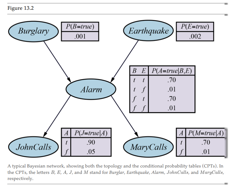
6. Bayes Nets
(chapter 13)
Bayes Nets (Bayesian Network) are a way to represent joint and conditional probabilities in a more succint and understandable manner. They give us access to different ways to greatly simplify the calculations required to perform inference, when compared to using full joint distributions.
It takes advantage of independance and conditional independance rules to do that.
A Bayes Net is a directed acyclic graph with quantitative probability information for each node. Definition:
- Each node is a random variable (discrete or continuous)
- Arrows connect pairs of nodes, from the parent (Y) to the child node (X).
- Each node X_i has associated probability information Theta(X_i | Parents(X_i))) that quantifies the effect of the parents on the node using a finite number of parameters
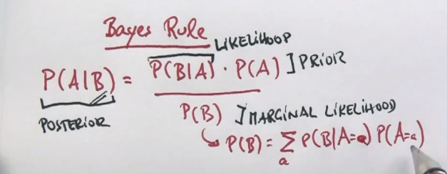
It is said that Cavity is a “Cause”, that is, it has a direct influence on its “Effects” (Toothache and Catch). It is accepted that Causes should be parents of effects.
This means that Toothache and Catch are considered conditionally independent. That is, if we don’t know the value of “Cavity”, then knowing the value of Toothache can influence our knowledge of Catch, and vice-versa. However, if we know the value of “Cavity”, then the value of “Catch” doesn’t give us more information about “Toothache”.
Alternatively, we also call the Cause/Parent “Not Observable” and the Effect/Child “Observable”. We know that we have a tooth ache, so what is the probability of a cavity with that knowledge? On the opposite side, the patient “knows” whether they have a toothache, trying to infer a toothache from the knowledge of a cavity is of little use.
Usually, domain experts will help with building the graph, as they know what random variables are causes to which effects.
How to use Bayes Rule to solve Bayes Nets? Naive formula:
$$ P(A|B) = \eta P’(A|B) = \eta P(B|A)P(A) $$ Where $$ \eta = P’(A|B) + P’(Not A|B) $$
Semantics of Bayes Nets
If the Bayes net contains n random variables X1, X2, … Xn, then the joint distribution is
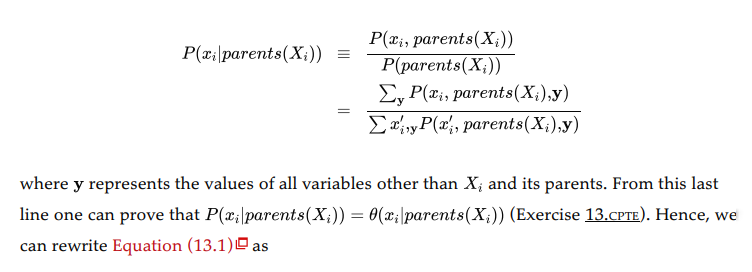
$$ P(x_1, x_2, …, x_n) = \prod_{i=1}^n P(x_i | parents(X_i)) $$
Building a Bayesian Network
“The Bayesian network is a correct representation of the domain only if each node is conditionally independent of its other predecessors in the nore ordering, given its parents. Here’s how to satisfy this condition:
- Nodes: Determine the variables that will be part of the domain. Then order them such that cause precedes effects (not necessary, but will help make the model compact).
- Links: For i = 1 to n do:
-
Choose a minimal set of parents such that the following is satisfied: $$ P(X_i | X_{i-1}, …, X_1) = P(X_i|Parents(X_i)) $$
-
For each parent insert a link/arrow from the parent to X_i
-
CPTs: Write down the conditionl probability table P(X_i|Parents(X_i))
In other words, the parents of X_i should be the nodes that directly influence X_i.
This method also ensures that we cannot create a Bayes network that violates the axioms of probabilities (since there are no redundant probabilities).
Explaining Away
The phenomenon where two independant variables in a Bayes Net are not conditionally independant. So if S and R are independant, then P(S|H) is not independant of P(R|H)
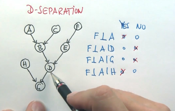
D-Separation
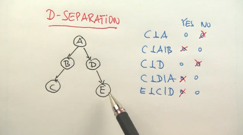
Any 2 variables are independant if they’re not linked by just unknown variables.
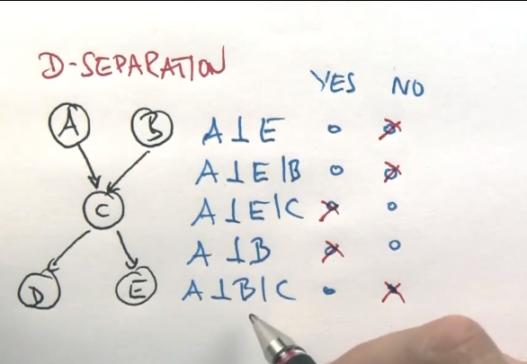
D-Separation or Reachability can be explained as such:
If all of A->B->C are unknown, then A and C are dependent. We call this an “Active Triplet”.
If A->B->C and B is known, then A and C become independent. We call this “Inactive Triplets”.
Similarly, if B->A and B->C, then A and C are dependent. However, if B was known, then A and C are independant.
If A->B and C->B, and B is known, then A and C are dependent. If B is unknown, then A and C are independant.
If A->B->…->F and C->B->…->F and F is known, then A and C are dependent.
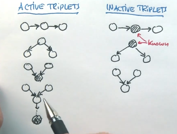
- A variable is conditionally independent of its other predecessors given its parents
- Each variable is conditionally independent of its non-descendants, given its parents.
- A variable is conditionally independent of all other nodes in the network, given its parents, children, and children’s parents (its Markov Blanket)
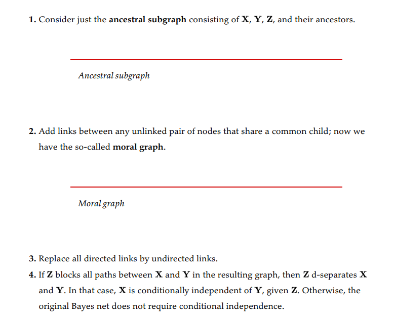
We can formally check for D-Separation as follows:
Exact Inference in Bayes Nets
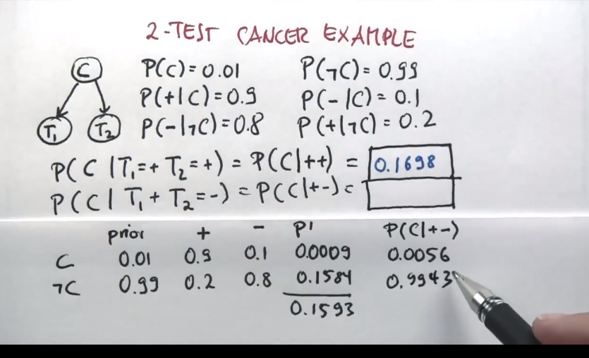
This section goes over the different algorithms that we can use to compute posterior probabilities, given an evidence.
Inference by Enumeration
The slowest algorithm, since it requires calculating the full joint distribution.
$$ P(X|e) = \alpha P(X, e) = \alpha \sum_y P(X, e, y) $$
Where E is the set of evidences e, Y is the set of unobserved variables y, and X is the query variable.
The term P(X, e, y) can be written solved using a product of all the conditional probabilities from the network. $$ P(x_1, x_2, …, x_n) = \prod_{i=1}^n P(x_i | parents(X_i)) $$
An example from the book:
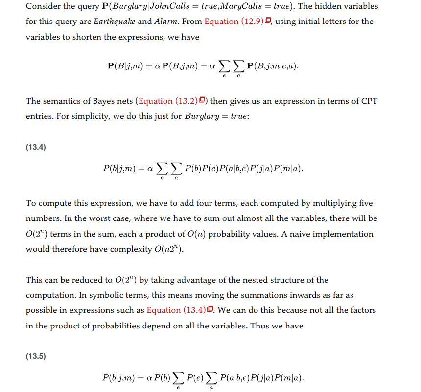
We can also represent the problem as a tree of probabilities:
Variable Elimination Algorithm
Complexity of Exact Inference
Exact inference can quickly become intractable based on the nature of the network (singly connected vs multiply connected as in the insurance example).
Clustering algorithms exist to reduce the complexity, but it also doesn’t always work.
Aproximate Inference for Bayes Nets
If the problem is too hard, we can resort to approximation, notably via random sampling methods (Monte Carlo algorithms).
They work by simulating a bunch of different scenarios based on the probabilities of each variable to occur. This can help recreate situations multiple times for us to compute the actual distribution.
7. Machine Learning
(chapter 19.1-19.5, 19.7, 20.1, 20.2)
Binary Classification
The linear equation for a decision boundary can be represented with vectors:
$$\overrightarrow{w} \cdot \overrightarrow{x} = 0$$
where the vector w is <b, weight of x1, weight of x2, …> and where the vector x is <x0, x1, x2, …>
Supervised Models
K-NN From each point in the training data, calculate distance from closest neighbors. The data point is assigned a class based on popularity vote. (chapter 19.7.1)
- Nonparametric
- Works great with dense data (low dimension, lots of data)
- Not good with classifying outliers
- But not very sensitive to outliers
Naive Bayes Calculate a conditional probability, given the class, for each class. The class is assigned based on the most likely (chapter 20.2.2)
- Very effective general purpose algorithm
- Scales well to large problems (2n + 1 parameters for n boolean attributes)
- Deals well with noisy or missing data
- Drawbacks: - The assumption is not often accurate - Doesn’t perform well with lots of attributes, it is often overconfident one way or another.
- Assumption: Attributes are conditionally independant of each other, given the class.
- Parametric, the parameters are (for boolean variables, 2 classes)
- Obtain probability of each class like this:
Decision Trees
Decision trees are built intuitively (try to split the data to get best accuracy). Issues arise with overfitting trees if we go too deep, so we try to tune for the depth parameter to generalize the tree.
We calculate the information gain for each node as such:
$$ Gain = B(\frac{p}{p+n} ) - Remainder(A) $$ Where $$ B(q) = -(q log_2(q) + (1-q)log_2(1-q)) $$ $$ Remainder(A) =\sum_{k=1}^d \frac{p_k + n_k}{p+n}B(\frac{p_k}{p_k+n_k}) $$ d is the number of distinct value for attribute A. p are positive examples n are negative examples
Another information gain function is known as the Gini gain, from Gini Impurity.
Random Forests
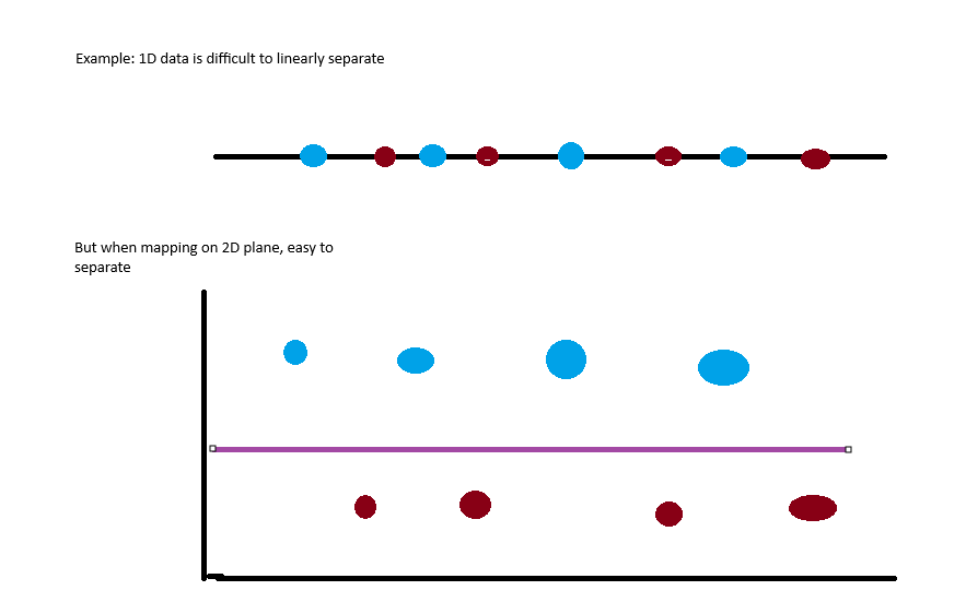
Support Vector Machine (SVM) (ch. 19.7.5
- Nonparametric
- Generalizes well
- Good for sparse datasets (Lot of dimensions, but not lot of values)
- Good when the data is not linearly separable in its dimensional space.
- Linearly separates data in a higher dimensional space.
- Class labels -1 and 1 instead of traditional 0 and 1
- Intercept is the separate parameter b
Unsupervised Models
Metrics
8. Pattern Recognition Through Time
(chapter 14, 23)
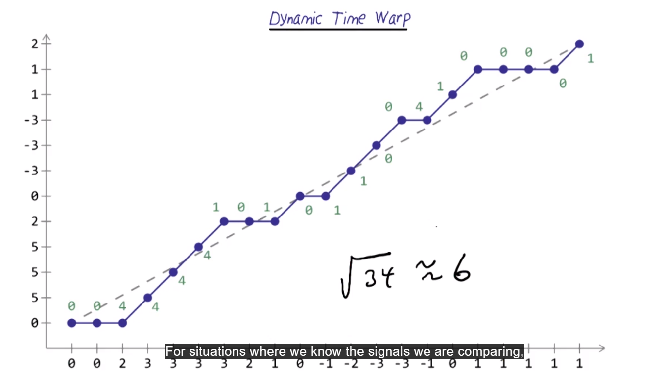
Dynamic Time Warping
(Lectures)
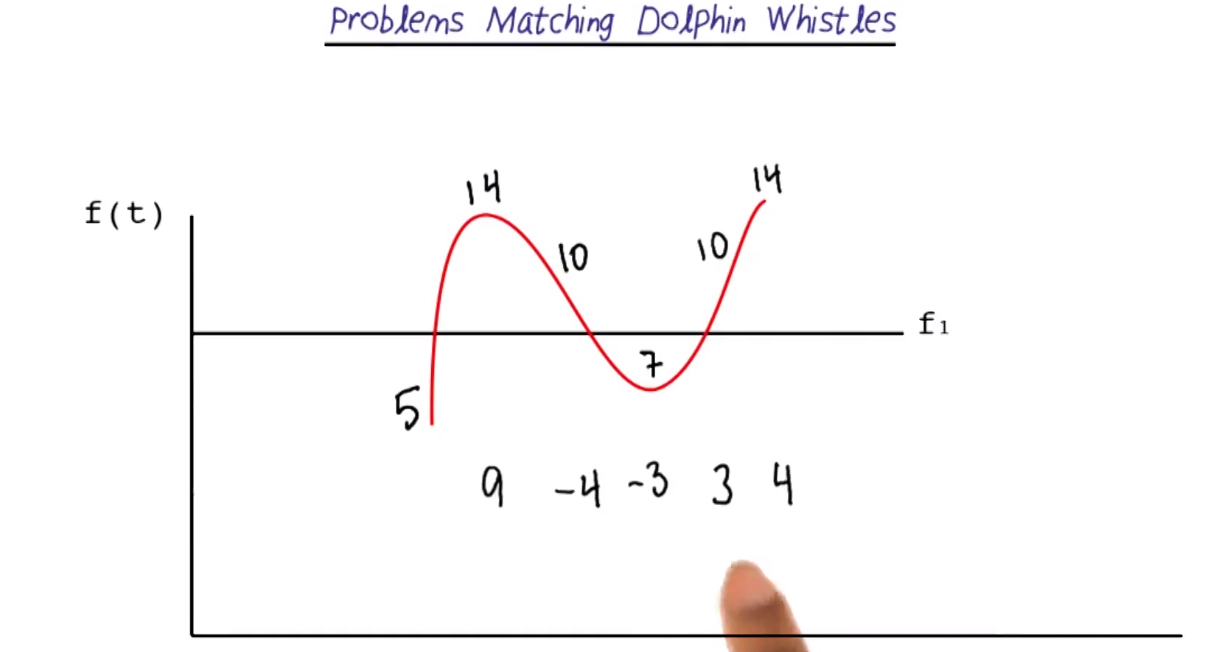
Problem matching is used to match different time-based signals. For example, the dolphin signals might have the same up and down patterns, but at different frequencies. So, we use “delta frequency”.
Let each “matched” data point be the delta between two consecutive points.
For warping, we try to align the two time series so they best match up - set the shorter signal on y-axis, and longer one of x-axis.
A perfect match would be a straight diagonal. Match pairwise elements in order to minimize the time warping. If a tie, try to match the diagonal.
Finally, calculate euclidean distance (or other measure of distance).
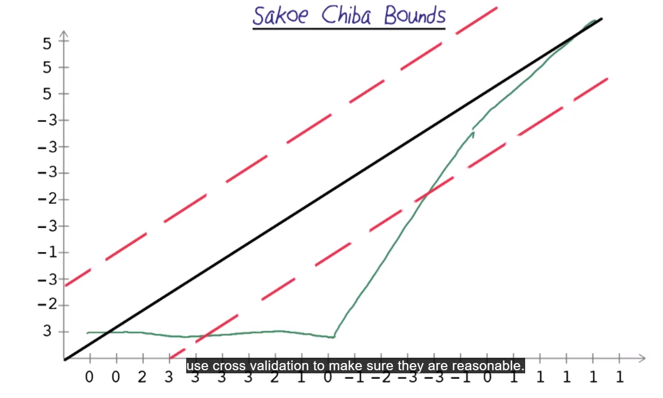
Sakoe Chiba Bounds
An issue with dynamic time warping, is that they might make two time series look closer than they are.
Sakoe Chiba bounds are used to force us to keep to the diagonal to an extent. Decide which bounds to use by testing different bounds and using cross-validation.
Formally
References the paper “DTW Myths” by Ratanamahatana and Keogh
Take two difference time series of length n and m
$$ Q = q_1, q_2, … ,2_n $$ $$ C = c_1, c_2, … , c_m $$
- Build an nxm matrix where each cell represents the squared distance (x - y)^2 between both.
- Recursively, starting from the top left, add the minimum of the “previous” cells touching the current one.
Formally, $$ DTW(Q,C) = min \sum_{k=1}^Kw_k $$ where w_k is the cell at (i,j)_k that also belongs to kth element of a warping path W.
Hidden Markov Models (HMM)
Consider first order MM, only depend on the state immediately preceding them.
- Used for recongnition in data with a language like structure.
HMM Representation
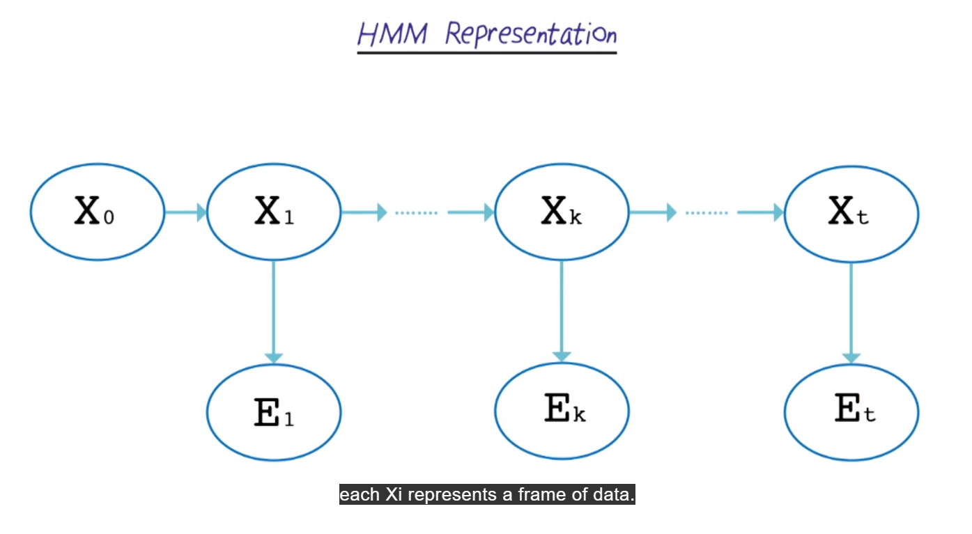
- X_i is a frame of data
- X_0 si the start state
- X_1 is the first time frame
- E_1 is the output at that time 1
- X_2 is the next time frame
- E_2 is the output at X_2
- etc. until the end of the sequence
Another representation
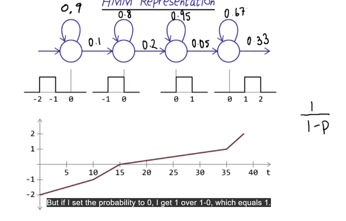
- Loops are self-transitions: Model can stay in the same state multiple times over with some probabilities
- Emission probabilities (or alpha probs) are the uniform distributions (which number can it be at each state)
- Transition probabilties: For example in state 1, there are 10 frames, so 10 “possibilities” of stating in state 1. So, we assign porbability of 1/10 for transitioning. Self transition has to be 0.9. Etc. for others.
- 1/(1-p) -> p is the self-transition probability. Helps find the number of time frames we expect to stay in one state.
- special: I the self-transition probability = 0, thenexpected frame=1. Because we enter the state, output an emission, then leave the state immediately.
- Add dummy state to explicitely enter the first state
Viterbi Trellis
- Outputs a probability that a squence of states belongs to one model or another
- Highest probability model is assigned the sequence
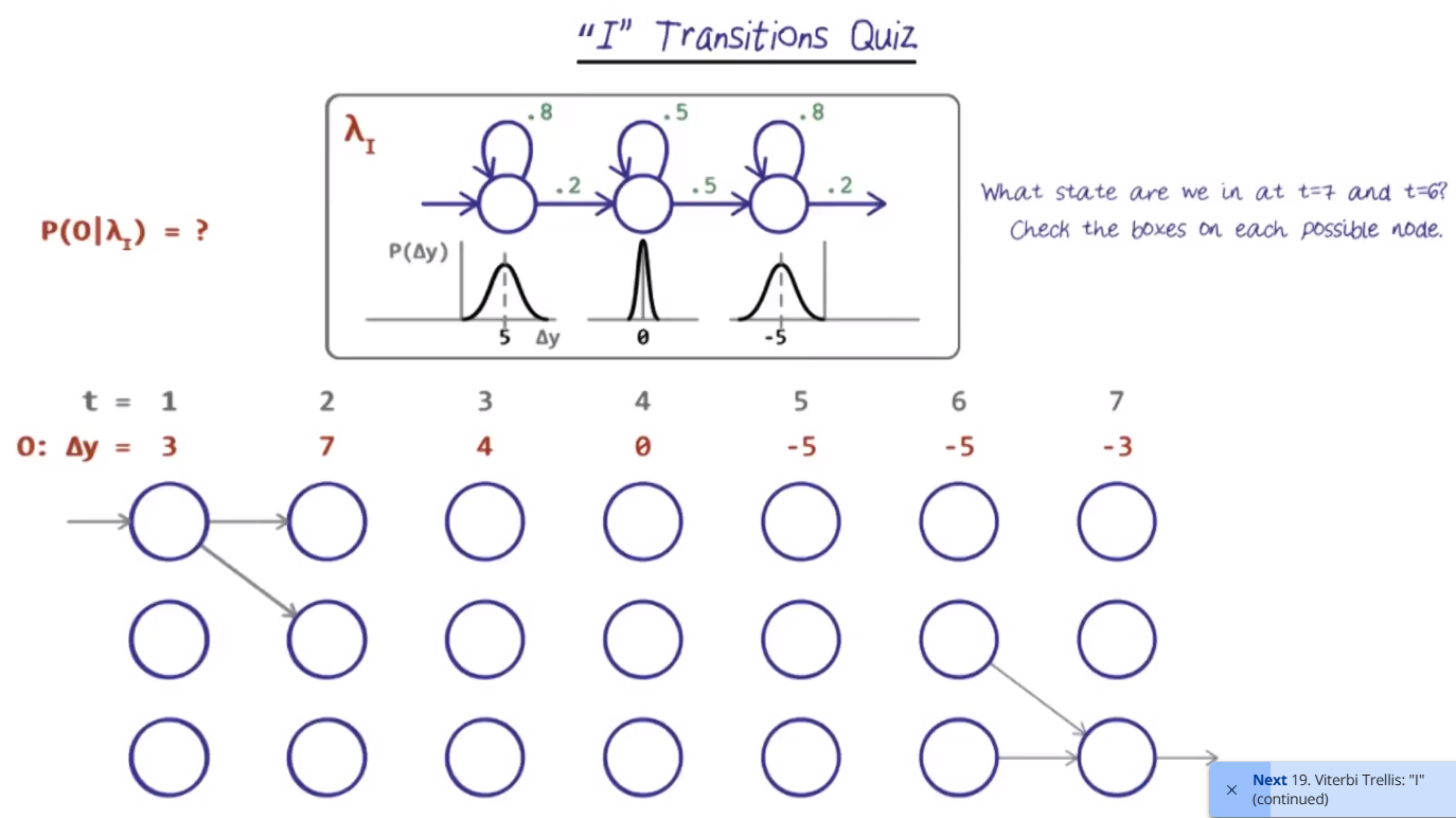
In this example, we know that we need to end at state 3. So the step prior (time 6) was in state 2, or 3.
Add transition probabilities for each state:
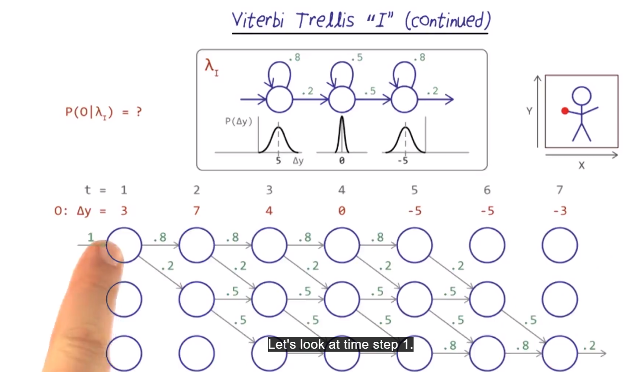
Overall probability
- In each node, figure the probability assigned to each delta-y (in the example, the number is made up, but using the gaussian distribution, estimate the P(delta-Y = 3) = 0.5
- In time 2,
- since 7 is the same distance from the mean of 5, we assume same probability (0.5)
- For state 2, we look using the probability at state 2
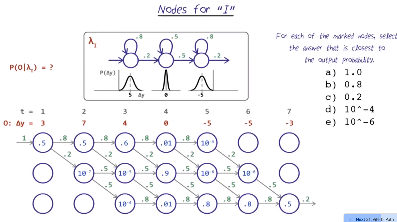
Viterbis Path
- Using all the filled probabilities, find the more likely by multiplying each node by its transition probability, and continue multiplying until the end
- Obviously this can become really small numbers
- Usually, use log based to avoid too small numbers
- For example: Transitioning from State 1 to State 2
- E(Staying in 1) = 0.8 * 0.5 (from time 2)
- E(going to State 2) = 0.2 * 10^-7
- Overall Path to State 1 at time 2: 1x0.5x0.8x0.5 = 0.2
- Pick the maximum such path
Planning and Logic
In other words, a |= b iff M(a) subset_or_equal M(b).
Where “M” is the world of b, the world of a - the model.
Propositional Logic: Truth Table
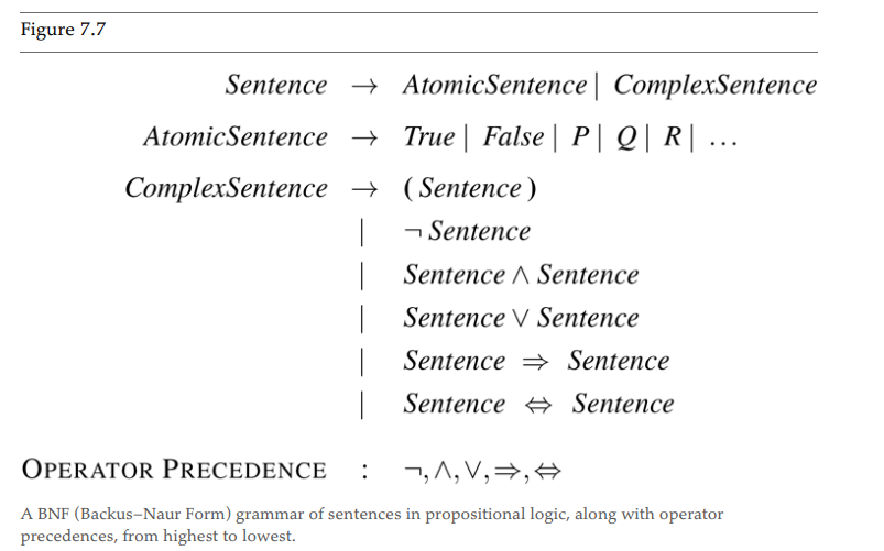
| P | Q | Not P | P N Q | P U Q | P -> Q | P<->Q | P XOR Q |
|---|---|---|---|---|---|---|---|
| False | False | True | False | False | True | True | False |
| False | True | True | False | True | True | False | True |
| True | False | False | False | True | False | False | True |
| True | True | False | True | True | True | True | False |
Where P->Q is “P Implies Q”. Meaning, “If P is True, claim that Q is True”. Which is True in both cases where P is false.
P<->Q is a biconditional, of iff. P is true iff Q is true. P is False iff Q is false.
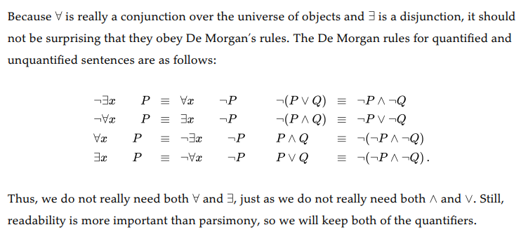
If a entails b and b entails a, then we say that a is equivalent to b. Some logical equivalences are:
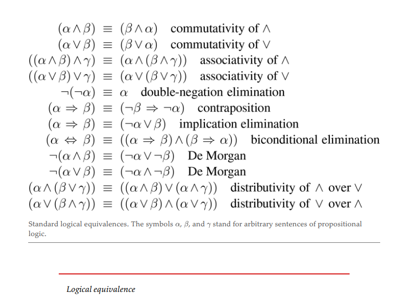
Proves One technique to solve proofs is to transform a sentence into a conjunctive normal form (CNF) - only clauses. Here’s how one can go about converting a procedure to CNF
Procedure -> CNF
- Replace bijunctions (<->) with two implications (a <-> b to a->b AND b->a)
- Replace implications with not(a) OR b (a->b becomes not(a) U b)
- Move negations inwards using logical rules
- Apply distributivity law whenever possible so that AND and OR operators aren’t nested.